15618 Project: Fibonacci Heap in Parallel
Final Report
Fibonacci Heap in Parallel
15618 Project Final Report
Members: Lemin Zhang (leminz), Zihao Du (zihaodu)
Summary
Our project focuses on implementing and parallelizing Fibonacci heaps for multi-core systems. We first developed a sequential baseline implementation as a correctness reference for later designs. We then explored two concurrent implementations based on coarse-grained and fine-grained synchronization. Based on the observation that locking and synchronization overhead can be reduced by partitioning the heap into smaller sub-heaps, we implemented a distributed, worker-partitioned design called MegaFib. To evaluate its practical usefulness, we built Dijkstra’s algorithm on top of MegaFib and benchmarked the system on both homogeneous and heterogeneous CPU platforms. This paper describes the design of each approach, analyzes its performance under different workloads, and discusses the tradeoffs involved in parallelizing heap operations.
https://leminzhang.github.io/projects/parallel_fib_heap/finalreport/
Background
Problem Overview
A priority queue is a fundamental data structure used in many graph and search algorithms, such as single-source shortest path, branch-and-bound search, and best-first search. Among sequential priority queue implementations, the Fibonacci heap is theoretically one of the most efficient data structures (Cormen et al., 1990; Fredman and Tarjan, 1987). However, its sequential design is not directly scalable on multi-core machines, because operations on the shared root list, minimum pointer, and tree structure can create synchronization bottlenecks.
This paper studies concurrent Fibonacci-heap-inspired priority queue designs for parallel execution on multi-core systems. Our goal is to understand whether and when heap operations can benefit from additional cores, and how different synchronization and partitioning strategies affect scalability. The main challenge is that priority-queue operations, especially minimum extraction, require coordination over shared state and can easily become serialization bottlenecks. Prior work on concurrent priority queues has shown that strict extraction semantics often increase contention, while relaxed or non-strict extraction can improve throughput when applications only require a high-priority element rather than the globally minimum one (Bhattarai, 2018; Huang and Weihl, 1991). However, in our work, a novel method is introduced to implement the Fibonacci heap, which has no relaxed extraction and could still achieve superior performance.
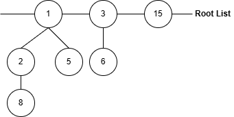 Fibonacci Heap Structure
Key Data Structures
A Fibonacci heap is a forest of heap-ordered trees. Each tree satisfies the minimum-heap property, meaning that every node has a key greater than or equal to the key of its parent. All tree roots are connected through a doubly linked list, called the root list. The heap also maintains a pointer to the minimum root, so the minimum element of the entire heap can be accessed directly. Compared with other heap structures, such as binary heaps, the Fibonacci heap is more lazy and flexible. Its trees do not need to follow a strict shape, the heap may even contain many singleton trees in some cases. The three core priority queue operations considered here are Insert, DeleteMin, and DecreaseKey. We explain below how the Fibonacci heap achieves its improved amortized running time.
Insert
The Insert operation takes O(1) amortized time. It is a very lazy operation: the heap creates a new node and added it into the root list next to the current minimum node. No tree merging is performed during insertion, which is why the operation only takes constant time.
This laziness also explains why the root list can become large and why the tree structure can become unbalanced. Instead of maintaining a strict global shape after every insertion, the Fibonacci heap postpones this cleanup work until DeleteMin.
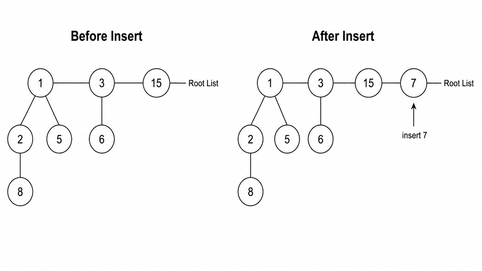 Fibonacci Heap Insert
DeleteMin
The DeleteMin operation is the most expensive operation in a Fibonacci heap. It takes O(log n) amortized time. The operation first removes the node pointed to by the minimum pointer. Then, all children of this minimum node are added to the root list, because after the parent is removed, those children become roots.
After this step, the heap performs a consolidation phase. During consolidation, roots with the same degree are repeatedly linked together. When two roots have the same degree, the root with the larger key becomes a child of the root with the smaller key, so the heap-order property is preserved. This process continues until no two roots have the same degree.
The implementation usually maintains an auxiliary array indexed by degree. Each array entry stores at most one root of that degree. When another root with the same degree is found, the two roots are linked, producing a tree with degree one larger, and the array is updated accordingly. The size of this array is O(log n) because the marking and cascading-cut rules of Fibonacci heaps guarantee that the maximum degree of any node is logarithmic in the number of nodes. Therefore, the amortized cost of DeleteMin is O(log n) (Cormen et al., 1990; Fredman and Tarjan, 1987).
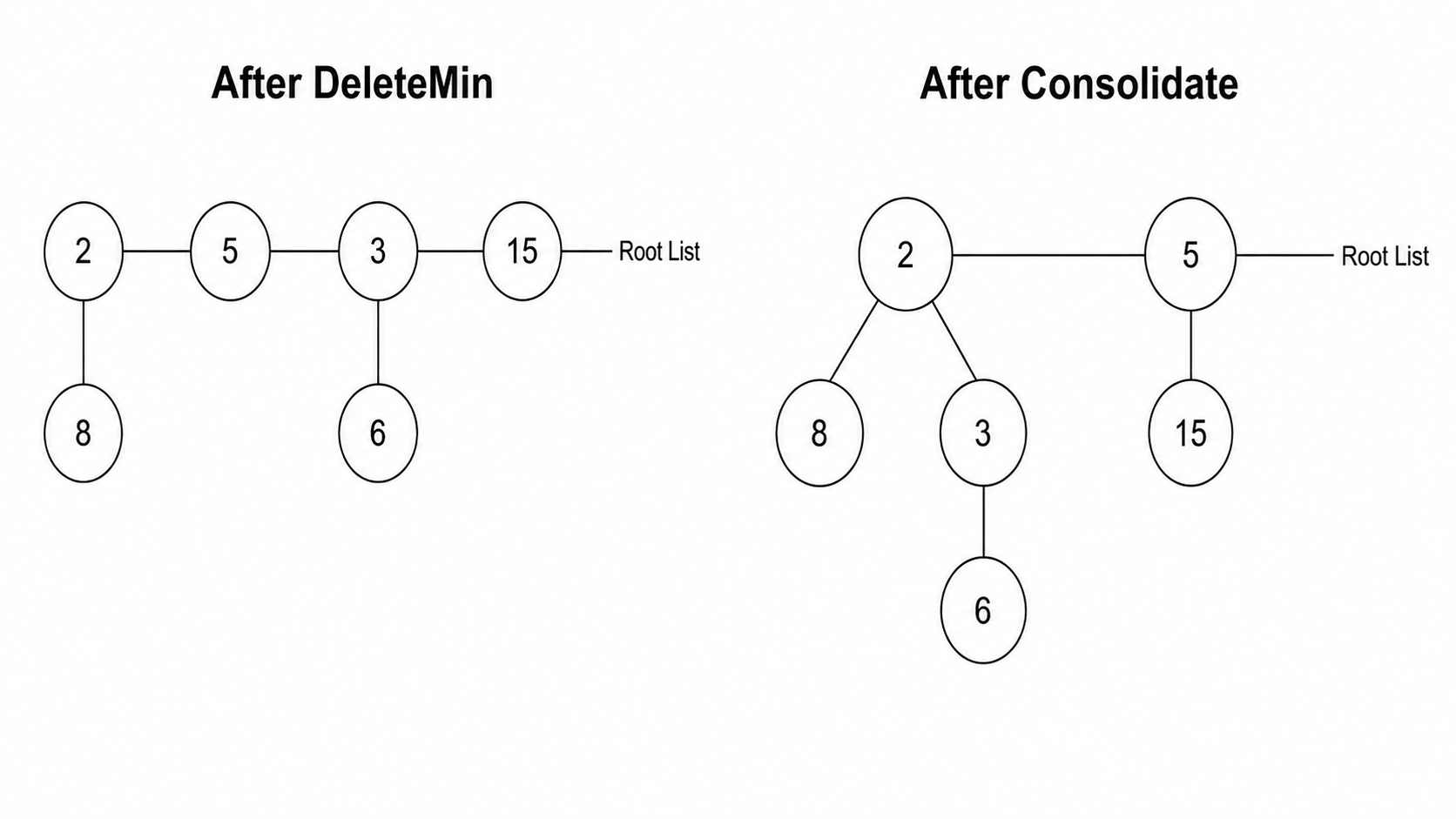 Fibonacci Heap DeleteMin & Consolidation
DecreaseKey
The DecreaseKey operation also takes O(1) amortized time. When the key of a node is decreased, we first compare the new key with the key of its parent. If the heap-order property is still satisfied, the tree structure does not need to change. However, if the decreased key becomes smaller than its parent’s key, the node is cut from its current tree and moved into the root list.
Repeated child removals can gradually destroy the structure needed to keep node degrees small. To prevent this, Fibonacci heaps use a marking mechanism. When a non-root node loses its first child, it is marked. If a marked node loses another child, it is cut from its parent as well, and the same rule is applied recursively to its parent. This process is called a cascading cut. The cascading-cut mechanism is a tradeoff between laziness and structural control: it avoids restructuring the heap too aggressively, while still preserving the logarithmic degree bound needed by DeleteMin.
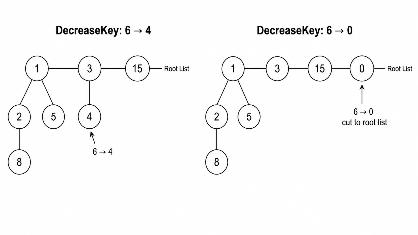 Fibonacci Heap Insert
Parallelization Opportunity and Workload
The main computational cost of a Fibonacci heap comes from operations that modify or scan shared heap structures. Although Insert and DecreaseKey have good amortized complexity in the sequential algorithm, they still need to update shared metadata such as the root list. The most expensive operation is DeleteMin, especially its consolidation phase. During consolidation, the heap scans the root list and repeatedly links trees with the same degree. This step involves pointer updates, key comparisons, and structural modifications, and it has O(log n) amortized cost. Therefore, DeleteMin and consolidation are the most obvious bottleneck for parallelization.
On the other hand, Insert is relatively easy to parallelize because it only adds a new singleton node into the root list. If the root list is divided into multiple sections, different threads can insert into different sections without competing for one global heap lock.
DecreaseKey also has some potential parallelism because many updates are local to the tree it belongs to. Significant performance gains can be achieved by parallelizing these operations with locks. DecreaseKey can also be approximated as inserting a new node with the decreased value while using version information to invalidate the old node (Brodal, 2022). This turns part of the operation into an insert-like workload, but it introduces extra stale nodes and can make later deletion or cleanup more expensive.
In contrast, DeleteMin has much stronger dependencies. A strict DeleteMin must return the global minimum, so concurrent delete operations cannot freely proceed without coordination. After the minimum node is removed, its children must be moved into the root list, and trees with the same degree must be consolidated. These steps modify shared root-list pointers and tree degrees, so that two threads cannot safely link or remove the same roots at the same time. This is the main reason why strict DeleteMin is difficult to parallelize. As demonstrated by prior parallel Fibonacci heap designs, one solution is to relax the extract semantics and allow an operation to return a sufficiently promising node instead of the exact global minimum, which reduces contention and exposes more concurrency. Another solution is to divide the heap into sections to allow the consolidation process to run in parallel. Although other processes in DeleteMin are kept sequential, this approach is still able to show superiority in parallel speedup.
Approach
Technologies Used
Language/APIs: The implementations were developed in C++17. Both the coarse-grained and fine-grained variants were implemented as thread-safe concurrent data structures. We used mutexes and shared locks for synchronization, and multiple worker threads executed heap operations concurrently to evaluate scalability under parallel workloads. In terms of parallelism tools, both Native POSIX Threads and OpenMP were used to implement the algorithm and run experiments. OpenMP Thread Affinity, giving us a detailed control on which work to run on which CPU core, was used to optimize the algorithm on heterogeneous CPU platforms.
Build System: We used make with a Makefile and the g++ compiler. Our OpenMP Thread Affinity setting requires a Windows platform to run.
Target Machines & Platforms: Some parts of the development were done on the Linux and MacOS platform, and other parts, especially the part with heterogeneous CPU, were done on Windows. The tests were performed on both the Linux and Windows platforms. The reason why the testing results on the MacOS platform were not used is that it is difficult to map a workload to a specific CPU core with MacOS, and the Mac machine used in development comes with a heterogeneous architecture, which makes it difficult to analyze the scalability. The details of those platforms are shown below.
| Characteristic | Values |
|---|---|
| Operation System | Ubuntu 24.04.3 LTS |
| CPU | Intel Core i7-9700 |
| Total Cores (Homogeneous) | 8 |
| Total Threads | 8 |
| Max Turbo Frequency | 4.70 Ghz |
| Processor Base Frequency | 3.00 Ghz |
| Hyper-threading | Not supported |
| RAM | 16 GB |
Details of the GHC Linux Platform
| Characteristic | Values |
|---|---|
| Operation System | Windows 11 |
| CPU | Intel Core i9-13900H |
| Total Cores | 14 |
| # of Performance-cores | 6 |
| # of Efficient-cores | 8 |
| Total Threads | 20 |
| Performance-core Max Turbo Frequency | 5.40 Ghz |
| Efficient-core Max Turbo Frequency | 4.10 Ghz |
| Hyper-threading | Supported on Performance-core |
| RAM | 32 GB |
Details of the Windows Platform
Implementation Strategies
Coarse-Grained Locking
The coarse-grained Fibonacci heap is the simplest thread-safe implementation of a Fibonacci heap. It directly wraps the sequential Fibonacci heap with a single global mutex, so each heap operation acquires the lock before accessing or modifying the shared heap state. Our sequential implementation follows the original Fibonacci heap design by Fredman and Tarjan (Fredman and Tarjan, 1987), which provides $O(1)$ amortized time for Insert, DecreaseKey, and FindMin, and $O(log(n))$ amortized time for DeleteMin.
Fine-Grained Locking
Our fine-grained Fibonacci heap implementation follows the general idea of prior relaxed concurrent priority-queue designs (Bhattarai, 2018; Huang and Weihl, 1991). We partition the forest into multiple sections so that different threads can operate on different parts of the heap with separate local locks. Inserts are distributed across sections, and consolidation is performed over sections at a time rather than under a single heap-wide lock. The implementation also maintains a shared promising list of candidate minima. In our design, decreaseKey is implemented through reinsertion, which simplifies updates but defers some cleanup work to the delete path. A more detailed description of the implementation is given below, and pseudocode is provided in Appendix A.
Insert
We insert K dummy nodes into the root list and use them to partition the forest into sections. The trees located between two neighboring dummy nodes form one section. Parallelism in the fine-grained design comes from this partitioning: instead of holding a global lock, each section is associated with its own local lock.
When a new node is inserted, the heap randomly selects one section and acquires that section’s lock, if the section is occupied, it will check another section. This design reduces contention on the insertion path and allows inserts targeting different sections to proceed concurrently.
The main overhead on the insertion path comes from maintaining the dummy-node section boundaries and acquiring the selected section lock. More broadly, the sectioned design also introduces additional management costs for candidate maintenance and delete-side coordination, which become important in less insert-dominated workloads.
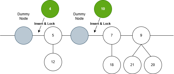 Insert Implementation
Spill-over
Since the heap is partitioned into sections, the current minimum is no longer maintained exactly in one globally synchronized location. To support relaxed deleteMin, we therefore use a spill-over procedure together with a shared promising list. The promising list stores a small set of candidate roots that are likely to contain low-key elements, so that deleteMin can usually avoid scanning the entire heap.
Whenever the promising list becomes almost empty, spill-over is triggered to refill all empty slots. In this process, the algorithm scans only a limited number of sections, collects root candidates from those sections, and keeps the smallest ones to refill the promising list. In this way, deleteMin does not need to examine the entire forest on every extraction, and the refill cost can be controlled by the number of scanned sections.
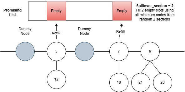 Spillover Implementation
The main advantage of spill-over is that it avoids a fully global minimum search and preserves scalability in insert-heavy workloads. However, this design also introduces a tradeoff. Because only part of the heap is scanned at each refill, the promising list may miss the true global minimum, so the returned deleteMin result becomes relaxed rather than exact. Increasing the number of scanned sections improves extraction quality, but it also slows the heap in delete-heavy workloads.
Consolidate
To control structural disorder in the sectioned heap, we periodically perform consolidation as a local maintenance operation. In our implementation, consolidation is not applied to the entire heap at once. Instead, one section is selected, we will do consolidate operation just like what we did in the sequential implementation in this section only.
The advantage of this approach is that it limits synchronization scope: consolidation repairs local structure without requiring a global heap-wide lock. This fits naturally with the sectioned organization of the fine-grained design. The tradeoff is that consolidation is no longer global, so it cannot fully restore the structural properties of a single unified Fibonacci heap. Consequently, the heap may retain cross-section disorder, and repeated local maintenance is needed to keep delete-side operations effective.
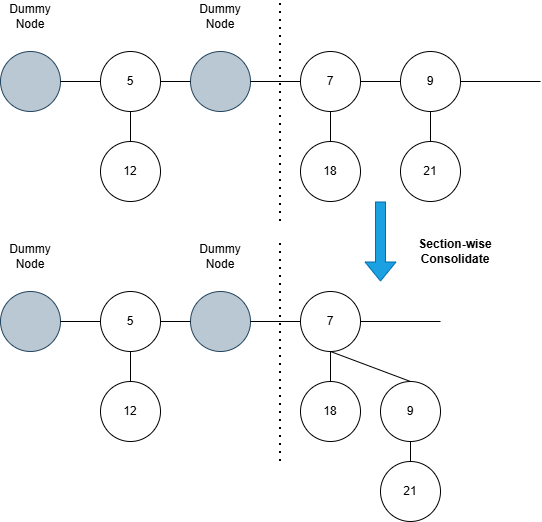 Consolidate Implementation
DeleteMin
As we mentioned above, deleteMin in our design is no longer an exact global-minimum extraction. Instead, it operates as a relaxed extraction procedure built around the promising list. When a deletion is requested, the algorithm first tries to remove a valid candidate from the promising list rather than searching the entire heap. If the selected node is an obsolete version created by a previous reinsertion-based decreaseKey, it is discarded internally and the deletion continues until a current version is found.
This makes deleteMin much more flexible than a traditional globally synchronized minimum extraction, since it avoids scanning and coordinating over the entire heap on every operation. However, the tradeoff is that deleteMin becomes both relaxed and maintenance-heavy. It may return a high-priority node rather than the exact global minimum, and it also absorbs the deferred cleanup cost introduced by stale nodes and local structural disorder.
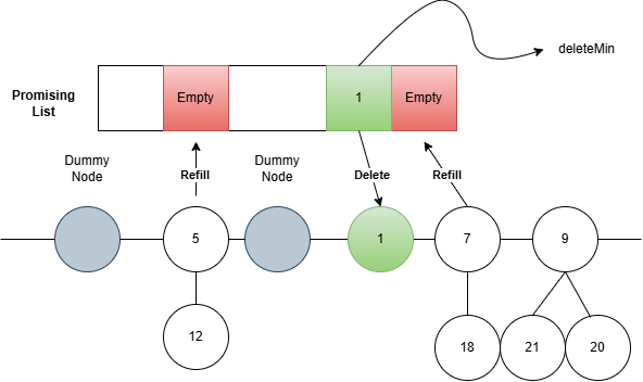 DeleteMin Implementation
DecreaseKey
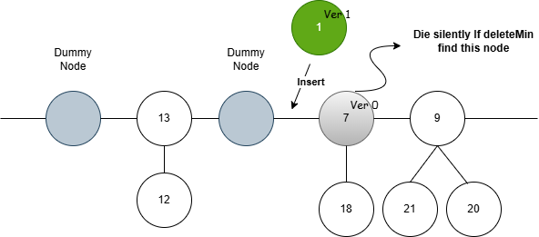
Because insertion in our sectioned design can be parallelized with relatively low overhead, we adopted a similar idea for decreaseKey. Instead of performing a traditional in-place decrease followed by possible cascading cuts, we implement decreaseKey through reinsertion – decreasing a key is treated as inserting a new node with the updated value.
To support this design, we maintain a shared generation table that records the current version of each live node. We increment the corresponding version and insert a new node with updated key and the new generation number. The main remaining issue is how to retire obsolete versions. We follow a lazy strategy: stale nodes are not removed immediately. Instead, during deleteMin, once a candidate node is selected, if the node is stale, it is discarded internally and the deletion procedure continues until a current version is found.
This design gives more flexibility than locking and updating an entire parent chain under cascading cuts. However, it also introduces an important tradeoff. Because obsolete versions remain in the heap until they are encountered by later deletions, the data structure accumulates stale nodes, which increases maintenance cost and further slows the delete path.
 DecreaseKey Implementation
MegaFib
MegaFib is a novel parallel Fibonacci Heap implementation aimed at improving the performance of all three heap operations, Insert, DeleteMin , and DecreaseKey for mega-scale heaps with hundreds of thousands of nodes. Large heaps are used in many scenarios, including shortest path founding for dense graphs. In heaps of smaller size, each heap operation is relatively simple, which means that it can be difficult to achieve significant speedup with parallelism since there are too few workloads to parallelize, and the performance gain will be neutralized by the overhead.
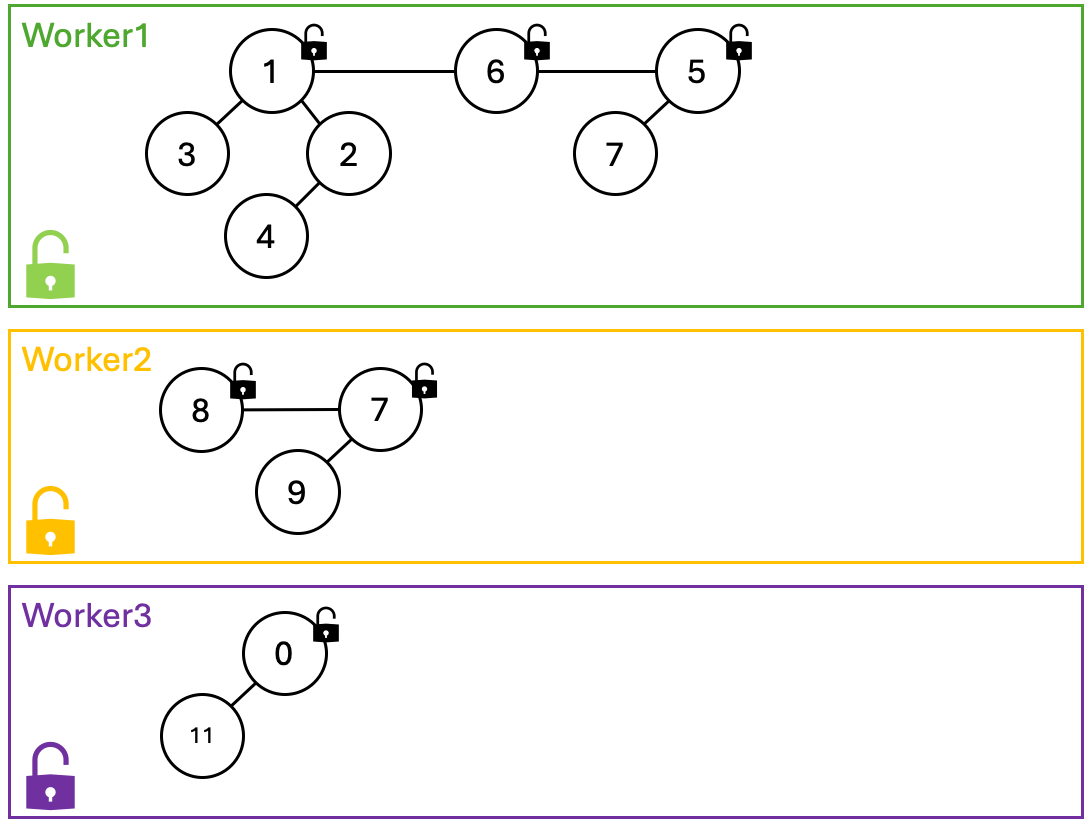
The basic data structure of MegaFib is shown in the figure below. For a system with $p$ threads, MegaFib consists of $p$ workers. There is an independent Fibonacci heap in each worker. The nodes in the heap are stored in only one worker at a time. Each worker has a mutex lock for synchronization, and each tree also has a lock. MegaFib has the same space complexity as the vanilla Fibonacci heap $O(n)$ where $n$ is the number of nodes in the heap. Different MegaFib workers need to maintain a balance of the number of trees to balance the workload of DeleteMin.
 Data Structure of MegaFib
MegaFib supports three different operations: Insert, DeleteMin, and DecreaseKey.
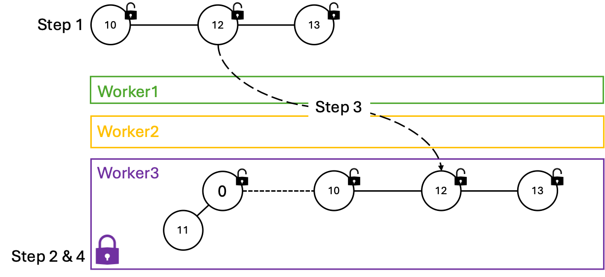
Insert: In our data structure, Insert on different workers is intrinsically parallel, since the heap on each worker is independent of each other. However, during development, we found that because the insert operation is so simple and fast, acquiring a worker lock for each inserted node takes much longer than actually inserting the node even without any synchronization conflicts. As a result, a batch insert method was introduced to leverage parallelism for performance, where the operation is divided into a few steps.
 Insert Operation of MegaFib
- Build a list of nodes for all the values to insert. No synchronization is needed, since this new list has no relationship to the heap yet.
- Select a heap worker to insert our nodes so that the balance of the number of trees is preserved as the maximum. Then acquire the worker lock.
- With the worker lock, we can perform any operations on the heap in the worker. As a result, it is safe to merge the existing list of trees with the list of new nodes we just built.
- Finally, release the worker lock, and all the values are inserted into the heap successfully. There is no need to main a pointer to the min node in MegaFib.
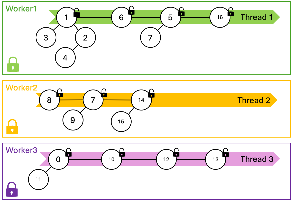
DeleteMin: The DeleteMin operation here is different from the vanilla implementation. Since MegaFib does not have a pointer at the min node to speedup insert, we need to find the min value first in DeleteMin. The detailed steps are listed:
 Finding Min and Consolidating Trees in DeleteMin
- Acquire all worker lockers. Since DeleteMin returns the global min value stored in the heap, we need to run the operation on a snapshot of it.
- Find the minimum value and consolidate the trees on each worker in parallel. Both finding the minimum value on a worker and consolidating the trees requires a traversal of all root nodes. As a result, those two tasks can be combined into one, which eliminates a $O(log(n))$ traversal of all root nodes.
- With the local minimum value on all workers, the global minimum value can be obtained by combining data from different workers. This step can only be performed sequentially without semantic relaxation.
- After finding the node containing the minimum value, that node needs to be deleted.
- Finally, the children, if any, of the deleted node need to be inserted back into the heap. Because the children of a node is stored in a list, there is no need to reconstruct a new list this time. All we need to do is insert the whole list of child nodes into a worker such that the balance of the number of trees on each worker is preserved as the maximum.
- All locks should be released after all operations have been performed.
DecreaseKey: The naive solution of the parallel DecreaseKey is to use the worker lock to perform operations on different workers concurrently. However, with this design, operations on different nodes of the same worker had to be performed sequentially. MegaFib does not compromise on this issue. Instead, a finer-grained locking mechanism is used. There is a lock for every tree in the heap. The majority of the DecreaseKey operation only needs to lock one tree of the node instead of the entire worker. However, in order to implement this algorithm, each node in DecreaseKey must know which tree it belongs to. There are two ways to solve this issue. On the one hand, the proactive way is that all nodes in the heap maintain a pointer to its tree root. On the other hand, the reactive way is that the node locates its root when its value is about to decrease. The first way would require much work when merging trees because this requires a traversal of all nodes in the child tree to change their roots. The second way only introduces overheads when the value of a node is decreased and its position needs to be changed. Since the tree merging operation is common in DeleteMin, the proactive way is likely to create more overheads, so MegaFib does it in the reactive way. Detailed steps are listed below.
- Find the root of all nodes with reduced keys. This step is carried out with worker by worker parallelism, and the worker lock is needed to ensure the heap structure does not change when the node is locating its root. As shown in the figure, thread 1 and thread 2 are responsible for finding the root of nodes with reduced key in their worker.
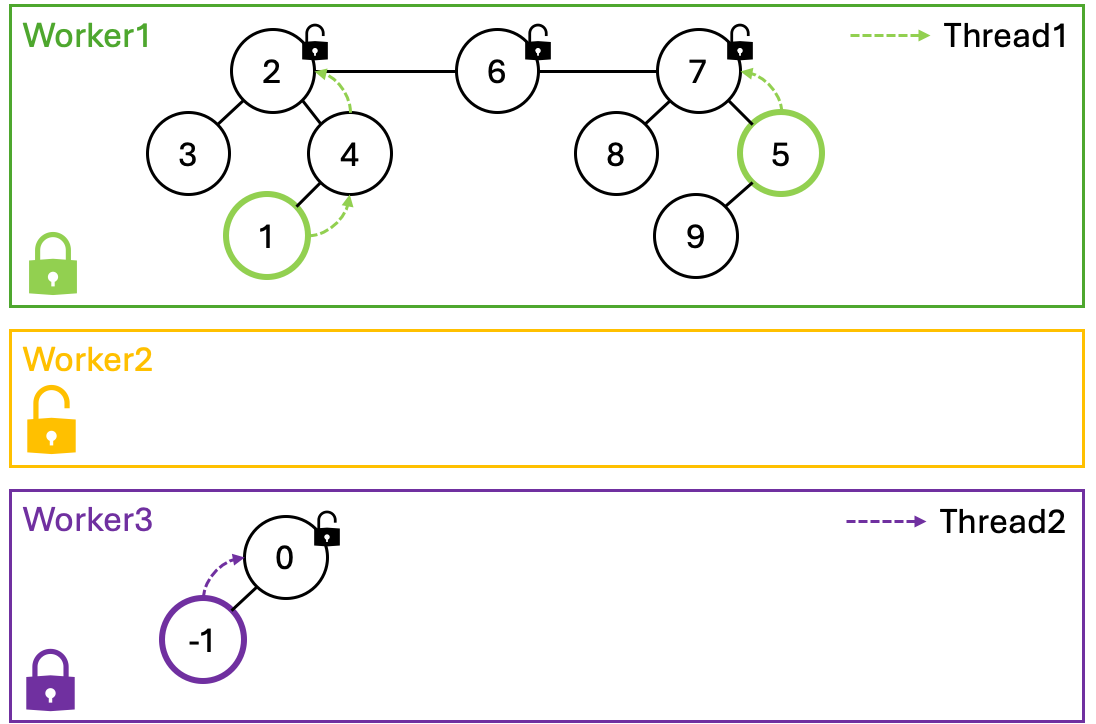 Step 1 of DecreaseKey: Finding Roots
- After the root of each node is located, the removal of nodes with decreased key and the construction of lists of nodes to be inserted back into the heap can be performed with tree by tree parallelism.
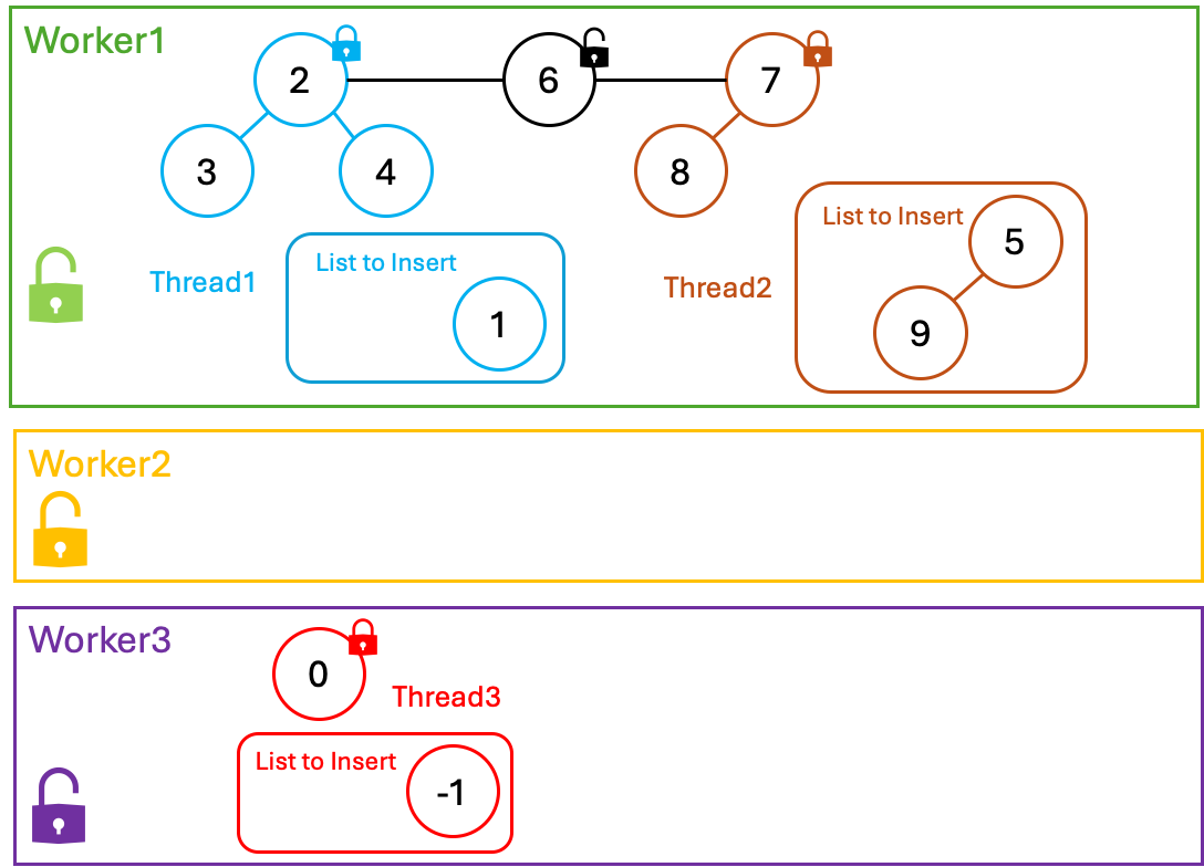 Step 2 of DecreaseKey: Tree by Tree Parallelism
- After the list of nodes to insert back to the heap is constructed, the insert operation will be performed with worker by worker parallelism.
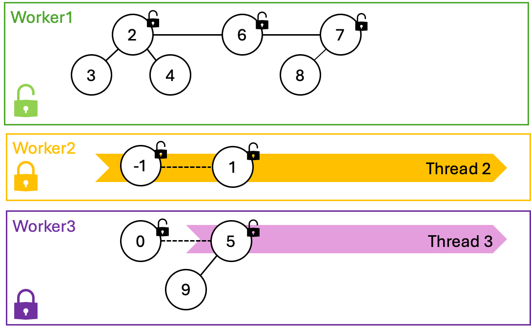 Step 3 of DecreaseKey: Insert Nodes back with Worker by Worker Parallelism
Benchmarking
Coarse and Fine-Grained Lock
Workload Generation
Trace generation was performed offline prior to timed execution. For each benchmark run, we first calculate the total number of operations and the target workload mix from user input, then generate a random operation trace using a random seed. The number of operations of each type was chosen to exactly match the specified workload ratios.
To avoid generating illegal operations, each step of the trace was sampled only from the set of operations that were currently valid. For example, deleteMin and decreaseKey were only generated when the heap was logically non-empty. This preserves the requested workload composition while ensuring that the trace remains executable.
We also used a warmup phase before timed execution. During warmup, we first inserted a base set of random keys, using 5,000 nodes to initialize the heap state. In addition, we inserted a protected set of handle-associated nodes reserved specifically for subsequent decreaseKey operations. These protected nodes were assigned large initial key values greater than 2,000,000, so that they would not immediately interfere with early deleteMin operations before being decreased. The handles corresponding to these reserved nodes were shuffled in random order, ensuring that decreaseKey operations were applied in a randomized but reproducible sequence. Regular insert operations generated random values in the range ([0, 1,999,999]); these nodes participated only in normal heap competition and were never selected as decreaseKey targets.
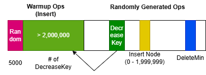 Random Trace Generation
After the trace is generated, the same trace is reused across all compared implementations. During timed execution, the trace is partitioned statically across worker threads, so that benchmark-side scheduling overhead is minimized, and performance differences primarily reflect the behavior of the heap implementations themselves.
| Parameter | Values / Description |
|---|---|
| Platform | Linux-based GHC machines |
| Threads | 1, 2, 4, 8, 16 |
| Operation counts | 10K, 100K, 1M |
| Delete-ratio sweep | (0.999, 0.001, 0.000); (0.995, 0.005, 0.000); (0.990, 0.010, 0.000); (0.980, 0.020, 0.000); (0.950, 0.050, 0.000) |
| Mixed decrease sweep | (0.990, 0.005, 0.005); (0.980, 0.010, 0.010); (0.950, 0.010, 0.040); (0.900, 0.010, 0.090); (0.800, 0.010, 0.190) |
| Representative insert-heavy workload | (0.999, 0.001, 0.000) |
| Representative mixed workload | (0.990, 0.005, 0.005) |
| Random seed | 42 |
| Warmup | 5000 random inserts + protected decrease-target nodes |
| Promising_size | 4, 8, 16 |
| Spill_sections | 1, 4, 8, 16 |
Experimental parameters.
| Metric | Description |
|---|---|
time_ms | Timed execution latency in milliseconds |
throughput_ops_per_sec | Executed operations per second; higher throughput indicates better parallel performance |
delete_value_sum | Sum of values returned by deleteMin; used as a coarse indicator of extraction quality, where larger values imply more relaxed semantics |
Performance metrics
Heap Locking Designs
We first compared three shared-heap designs across different thread counts: a coarse-grained locking Fibonacci heap, a fine-grained locking Fibonacci heap, and a binary heap baseline. The coarse-grained design protects the shared heap with a global mutex, effectively serializing all heap operations inside a single critical section. As a result, we expect its performance to degrade as thread count increases due to lock contention. By contrast, the fine-grained design attempts to reduce contention by allowing greater concurrency along the insert and decreaseKey paths and by limiting the scope of synchronization within the shared heap. For insert-dominated workloads, we therefore expect the fine-grained design to achieve higher throughput as more threads are added.
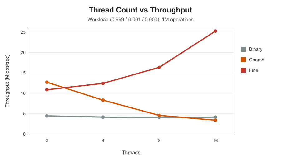 Throughput under an insert-dominated workload
The insert-dominated figure shows a representative success case for fine-grained locking. Under workload (0.999, 0.001, 0.000) with one million operations, the fine-grained heap continues to improve as thread count increases, rising from 10.82M ops/s at 2 threads to 25.29M ops/s at 16 threads. This result supports our expectation that, in an insert-heavy regime, the fine-grained insert path can exploit available parallelism effectively. In contrast, the coarse-grained heap degrades steadily from 12.72M ops/s to 3.38M ops/s as thread count increases. Its throughput eventually falls slightly below that of the binary heap baseline, which is implemented as a shared binary heap protected by a global lock. This behavior is consistent with increasing contention on a shared critical path.
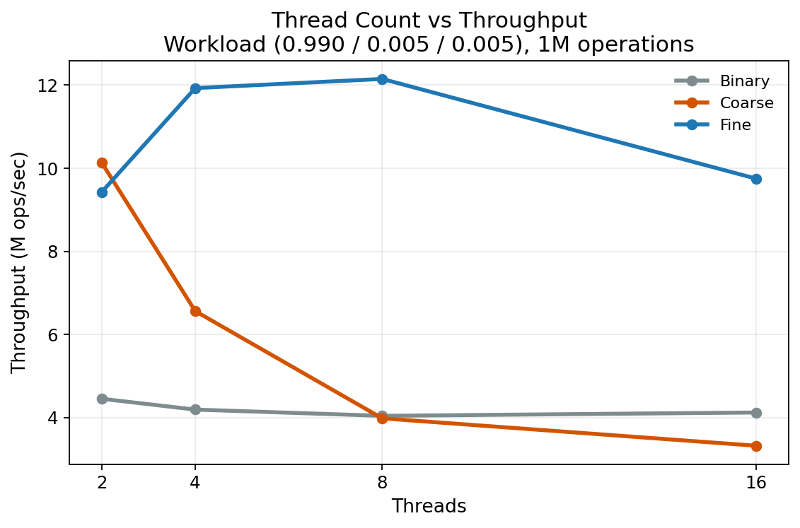 Throughput under a mixed delete/decrease workload.
The mixed workload figure shows a more demanding workload, (0.990, 0.005, 0.005), which includes both deleteMin and decreaseKey. Here the fine-grained design still outperforms the baselines and reaches 12.15M ops/s at 8 threads, but the trend is no longer monotonic: throughput drops to 9.75M ops/s at 16 threads. By comparison, the coarse-grained heap again declines smoothly as thread count increases.
Since our experiments were run on an 8-core GHC machine, the 16-thread configuration exceeds the number of physical cores. Since we run the experiment on GHC machine with Intel i7-9700, an 8 core CPU, we therefore expect the 16-thread results to be influenced by additional contention for hardware resources such as caches and execution units. This likely contributes to the throughput drop observed at 16 threads, particularly for workloads that already stress the shared synchronization path.
Taken together, these representative workloads show that our fine-grained lock design is beneficial, but only within a limited operating regime. It performs best when inserts dominate execution, yet we are not sure about its scalability.
Workload Sensitivity of Fine-Grained Locking
To better understand when fine-grained locking stops scaling, we varied the workload composition and conducted experiments on them. This isolates the behavior of the fine-grained heap itself and helps identify the conditions under which its shared coordination path becomes dominant.
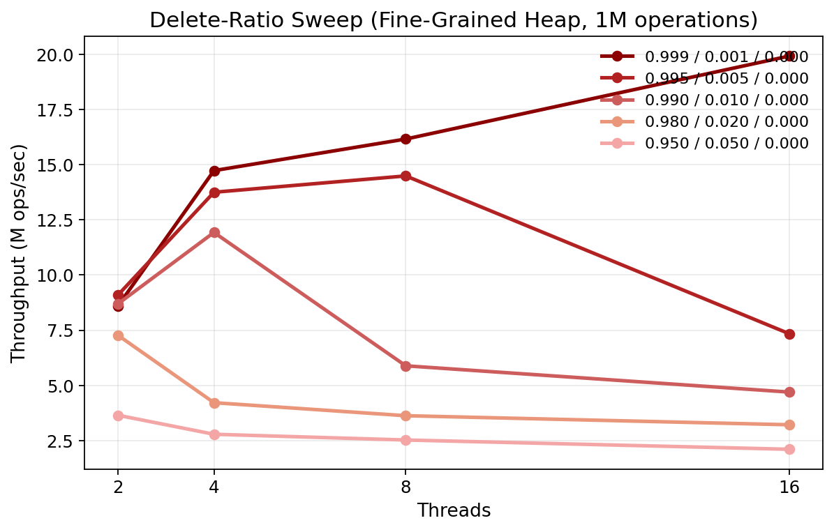 Delete Ratio Sweep
The delete-ratio sweep figure varies the deleteMin ratio while keeping decreaseKey=0. The main result is that the scalability turning point shifts steadily toward lower thread counts as delete pressure increases. For workload (0.999, 0.001, 0.000), the fine-grained heap still improves through 16 threads. For (0.995, 0.005, 0.000), the best point shifts to 8 threads. For (0.990, 0.010, 0.000), the best point occurs at 4 threads, and for heavier delete ratios such as (0.980, 0.020, 0.000) and (0.950, 0.050, 0.000), the best result already occurs at 2 threads. This is strong evidence that the shared deleteMin path, rather than the insert path, is the main limit to scalability. Under deletion-heavy workloads, multithreading no longer improves performance; instead, additional threads introduce more synchronization overhead and make the fine-grained heap slower than its lower-thread configurations.
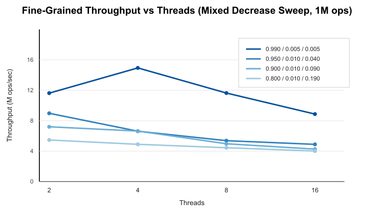 Decease Ration Sweep
The decrease ratio sweep figure complements this analysis by increasing the amount of decreaseKey work. The same leftward shift of the performance optimum appears here as well, but in some cases it occurs even earlier. For (0.990, 0.005, 0.005), the best throughput is achieved at 4 threads. For heavier mixed workloads such as (0.950, 0.010, 0.040), (0.900, 0.010, 0.090), and (0.800, 0.010, 0.190), the peak throughput degrades even more. Since these workloads fix a nontrivial amount of decreaseKey work, they suggest that reinsertion, version tracking, and delete-side cleanup all contribute to the same shared bottleneck.
Parameter Sensitivity of Fine-Grained Locking
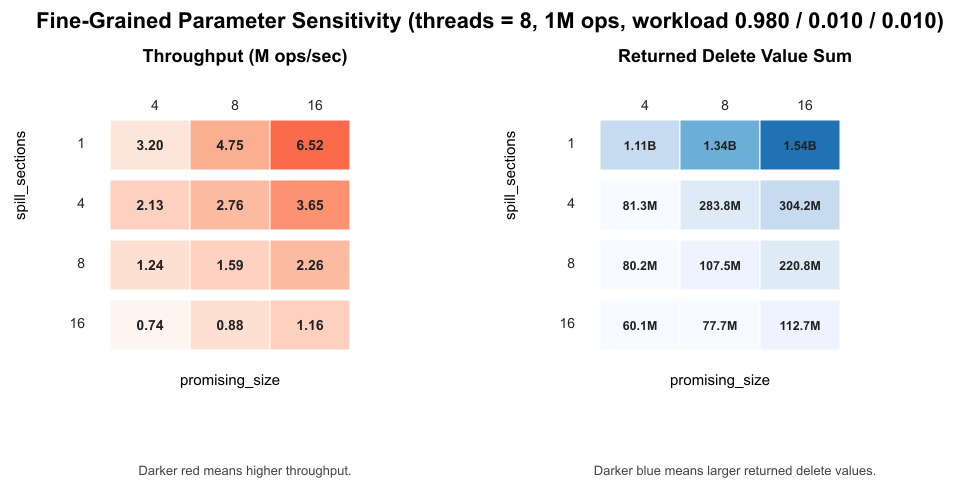 Sensitivity to candidate-pool and section-coverage
The figure above shows two clear relationships. First, spill_sections is the dominant throughput bottleneck: increasing section coverage sharply reduces performance. For example, with promising_size=8, throughput falls from 4.75M ops/s at spill_sections=1 to 0.88M ops/s at spill_sections=16. Second, increasing promising_size improves throughput in the current implementation, likely because a larger candidate pool amortizes refill and maintenance overhead.
The same figure also shows the corresponding tradeoff in returned deleteMin quality. Larger spill_sections reduce delete_value_sum, indicating that extraction becomes less relaxed and more accurate, but this comes at substantial throughput cost. Thus, the fine-grained Fibonacci heap design exposes a clear performance-quality tradeoff: narrow section coverage favors throughput, while broader coverage improves extraction quality but amplifies synchronization and maintenance overhead.
These sensitivity results reinforce the conclusions from the workload sweeps. Fine-grained locking is not ineffective, but its scalability is highly regime-dependent and remains constrained by shared coordination around delete-oriented work. Even in the workloads where it clearly outperforms the other methods, this speedup comes with a tradeoff in extraction quality, since higher throughput is associated with more relaxed deleteMin behavior.
Together, these observations motivated our next step: replacing the current shared-heap organization with a distributed heap design that reduces cross-thread interference on the global critical path.
MegaFib Benchmarking
For MegaFib, to gain a close insight into the performance of each operation, the three operations of the heap (Insert, DeleteMin , and DecreaseKey) are individually benchmarked. All results in this section were obtained from the GHC platform.
Insert
To benchmark insertion on MegaFib, we used a relatively simple demo workload. The workload is simply to insert a number of values into the heap. With lazy insertion of the Fibnonacci Heap, the specific value inserted makes no difference to the insertion performance.
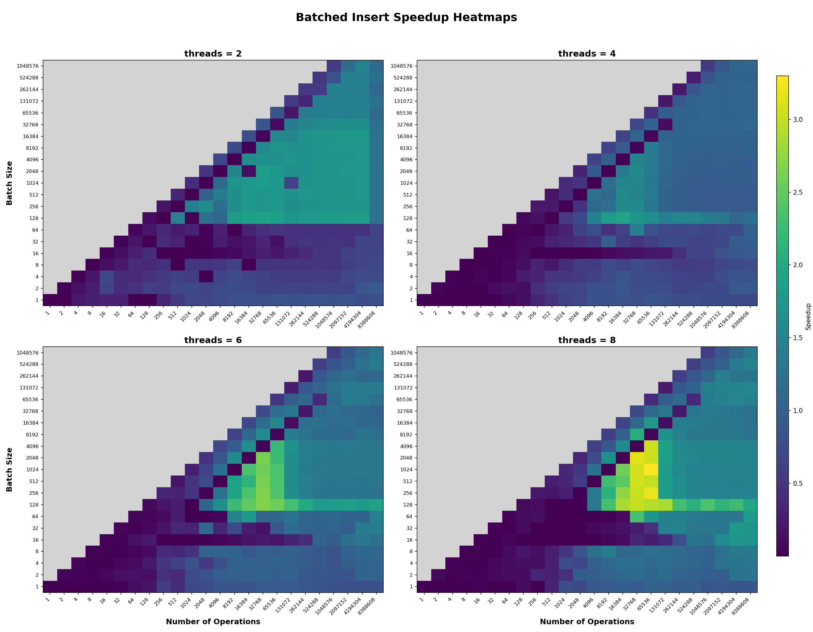
Batched Insertion is used in MegaFib, which makes batch size a very important parameter. The following figure shows the speedup with different batch sizes and numbers of operations (specifically, number of insertion here) for different number of threads. Some insights can be drawn from the figure. There is a triangle area with better speedup on the heat map for different thread settings, which we refer to as the “golden triangle”. The explanation of that triangle is shown in the discussion below.
 Insertion Speedup over Different Batch Sizes for Different Workload Size
- When the number of batches to insert is smaller than the total number of threads, MegaFib has very poor performance. This is easy to understand, since all nodes in a single batch will be assigned to only one worker. When the number of available workers exceeds the number of batches to run, there will be idle workers. Additionally, setting the batch size larger than the number of operations to run makes no sense, which are not included in the benchmark here and are marked gray in the figure. Only with enough batches to run can MegaFib balance the workload and obtain a performance improvement. This bound of number of batches to run forms the hypotenuse of the “golden triangle”.
- MegaFib only gets performance speedup when the batch size becomes large enough to neutralize parallelism overhead. Even with OpenMP, assigning a work to a specific thread has an overhead. As a result, if the work itself is too simple and fast, the performance gain from parallelism would be offset by those parallel overheads. Each batch is assigned to a thread as a whole OpenMP work, as batch size increases, the workload also increases, but the overhead to assign work does not change. Eventually, the speedup from parallelism would be able to offset the overhead, resulting in a positive overall speedup. This batch size limitation forms the bottom boundary of the “golden triangle”.
- The number of nodes to insert also plays an important role in the overall performance. As shown in the figure, if the number of operations is too large, MegaFib also struggles to obtain an optimal performance improvement. This is related to the memory hierarchy. As shown in the figure, when the number of values to insert exceeds 65k, parallel speedup drops significantly. One possible explanation is that the number of nodes is too large to fit in the cache and the processor has to drop some nodes into the RAM, which introduces many capacity cache misses. This memory hierarchy limitation is believed to form the right boundary of the “golden triangle”.
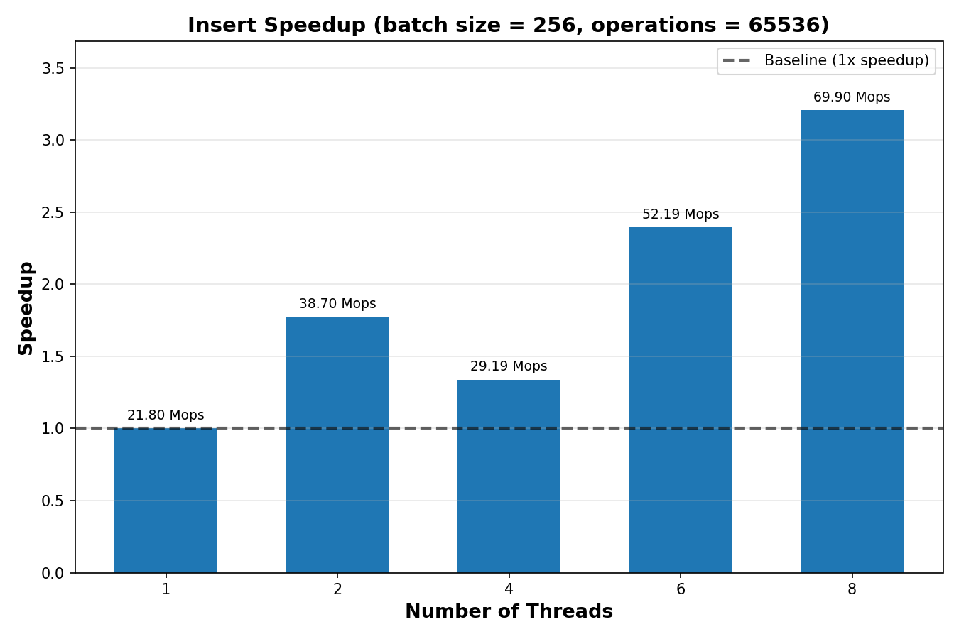
The figure below shows the throughput and speedup within the “golden triangle”. As shown in the figure, the parallel heap was able to achieve an insertion throughput of near 70 M operations per second, which is a speedup of 3.2x. Though this result is still far below linear speedup, it is still remarkable given that our workload has huge memory footprints and the computation for each operation is too simple to fully neutralize the overhead from parallelism.
 Insert Speedup and Throughput of MegaFib
DeleteMin
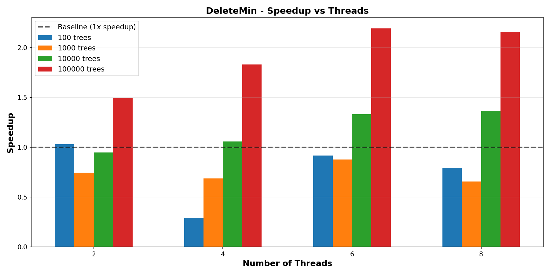
For the DeleteMin operation, the performance bottleneck is the $O(n)$ traverse of all trees in each worker to consolidate trees and find the minimal value. As a result, the running time of the operation depends mainly on the number of trees currently in the heap. To build a heap with so many trees, an insertion operation with a very large input size was performed, which generates a heap containing many trees with only one node in each of them. The number of nodes in a tree does not directly influence the DeleteMin operation, so simple trees with only one node were used. After the first DeleteMin operation consolidates the tress, the number of trees in the heap decreases dramatically, and the running time for the second operation will depend on the number of trees at that time. As a result, only the running time of the first DeleteMin operation is measured. The result is shown in the figure below.
 DeleteMin Speedup with Different Number of Trees in the Heap
As shown in the figure, the speedup differs a lot with a different number of nodes in the heap. When the number of nodes in the heap is small, the speedup is not stable. This issue is similar to what we have encountered in insertion. With too few nodes to process for each OpenMP work, the performance gain from parallelism could be offset by the overhead to start, end, and schedule works, making the calculated speedup irrelative to the heap operation load. With about 10000 trees in the heap, MegaFib was able to achieve a steady performance improvement. With about 100000 trees in the heap, the speedup of MegaFib became even better. Although the resulted speedup was below linear, the limited computation in our workload still makes this result considerably good.
DecreaseKey
In order to make a fair comparison on the performance of the Decrease Key operation over different threads used, a decrease test on all nodes in a fully consolidated heap was performed. This testing workload is similar to what the heap will encounter in application scenarios like shortest path algorithms making the result meaningful for real-world use. Detailed throughput and speedup are shown in the figure below.
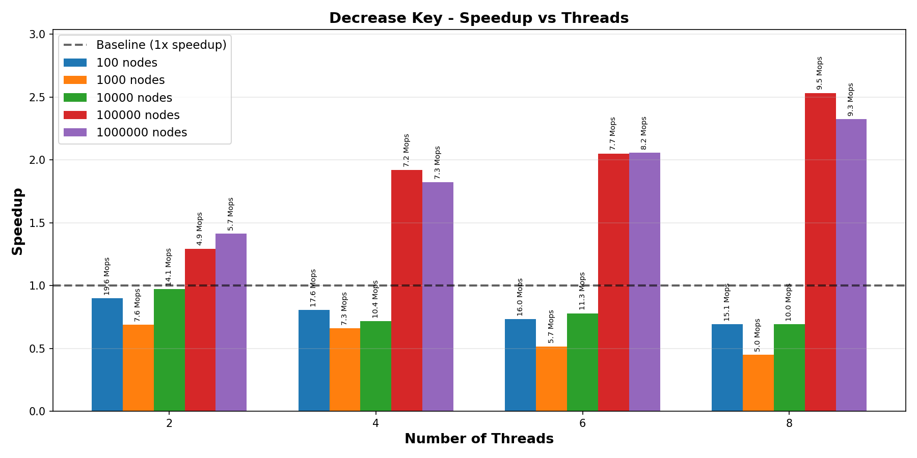 DecreaseKey Speedup and Throughput of MegaFib
As shown in the figure, speedup was small (less than 1) but the throughput was high when the number of nodes in the heap is relatively small. This can be explained again with the huge memory footprint of our program. When there were less than 10k nodes in the heap, a very large part of the heap can be put inside the cache. However, during the DecreaseKey operation, the memory access of each thread is highly random. For the Insert and DeleteMin operations, each thread only accesses data in its responding worker. However, our implementation of DecreaseKey runs with tree by tree parallelism, making the memory access pattern completely random. One tree accessed by this processor could be access next by a totally different processor. When the number of nodes in the heap is small, a lot of data can be kept in the cache. Tree by tree parallelism will introduce a ton of coherence cache misses and make the performance even worse. However, the situation with more nodes is different. Here, most cache misses are capacity misses, though tree by tree parallelism will still cause some coherence misses, its negative impact on the overall performance is offset by the performance gain from parallelism.
Dijkstra with MegaFib
A comprehensive benchmark was used to measure the performance of MegaFib in more realistic scenarios. One of the most import common usages of mega-scale heap is shortest path computation in dense graphs. For a fully connected graph with about 10000 nodes, there will be about 10000 values stored in the heap at the beginning. The performance of shortest path algorithms largely depends on the performance of the underlying heap.
In this section, a Dijkstra algorithm was implemented on MegaFib to compute the minimal distance for all nodes for a given graph. In order to demonstrate MegaFib’s ability to handle mega-scale data on the heap, a large fully connected graph with random distance on each edge was used as a test input. Since our goal is to evaluate the performance of the Dijkstra algorithm, only the shortest distance time was measured. The resulted performance is shown in the figure below.
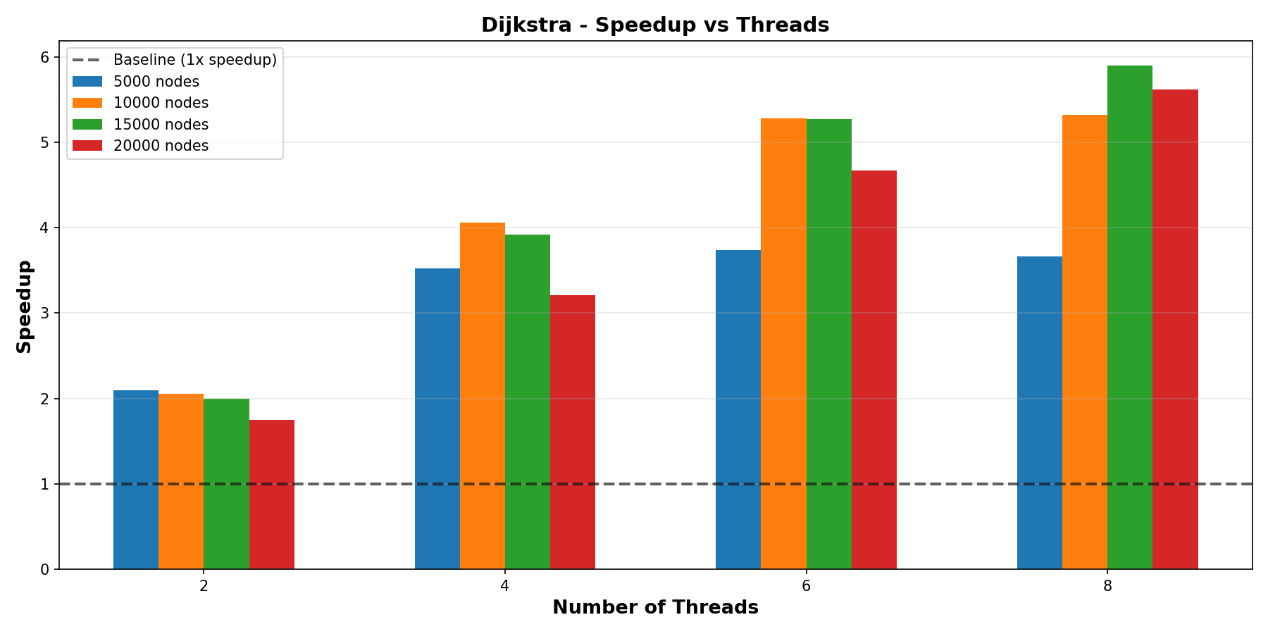 Speedup of the Dijkstra Algorithm with MegaFib on Fully Connected Large Graphs
Here a very steady speedup is achieved by our Dijkstra algorithm with MegaFib for different graph sizes. For smaller graphs, the algorithm was able to achieve nearly linear speedup with limited threads, but the scalability is worse. For instance, with 5000 vertices in the graph, the algorithm was able to achieve an over 3.7 speedup with 4 threads. Actually, the speedup for 10000 nodes is even larger than 4 for 4 threads. It is possible that the increase of high-level cache capacity caused this super linear speedup as more data can fit in this cache level. On the other hand, for large graph, the speedup of the algorithm with limited threads is not optimal, but the scalability was great. For example, with 20000 vertices in the graph, the speedup increased constantly as the number of threads went from 2 to 8. This phenomenon can be explained with the memory hierarchy. When the size of the graph was small, almost everything can fit inside the cache. Increasing the number of threads will increase the size of the high speedup cache usable, which will improve the performance. Nevertheless, too many threads running the same time will cause issues with coherence cache misses, dragging the overall performance. For large graph, most of the graph has to be put inside the memory. The program becomes more memory bounded, and the speedup is generally smaller. However, since the main memory does not have a coherence problem, when the number of threads is larger, the speedup is still steady.
MegaFib on Heterogeneous Architecture
All experiments in this section were performed on the Windows platform. The experiment setting was similar to section 3.2. The only difference is that since the machine we were using has only 6 P-cores (Performance Cores) and each P-core supports two threads, we tested running with 3, 6, 9, and 12 threads for P-core only experiment. Here, running with 3 threads means running with both threads of the first core and the first thread of the second score. Running with 6 threads means running with all threads in the first three cores. So on and so forth.
As shown in the figure below, the same benchmark test was run on the heterogeneous architecture. The subfigures on the left shows result with only P-cores and the subfigures on the right shows result with only E-cores (Efficiency Cores). The speedup with only E-cores was worse than the result on GHC machines. The speedup for P-cores was generally even worse than E-cores especially when the number of nodes in the heaps is small. However, as the number of nodes increases, we were still able to obtain some above 1 speedup on E-cores and P-cores. The result shows that the introduction of core affinity programming comes with a significant work management overhead. Only in experiments with enough computation for each OpenMP work (e.g. large number of nodes to process) can a speedup be observed. We have planned to optimize MegaFib on heterogeneous architectures. However, with this huge overhead for heterogeneous programming, it is difficult for such optimization to bring real performance improvement. Our workload is so simple and fast that the use of heterogeneous programming tools becomes an obstacle rather than an advantage.
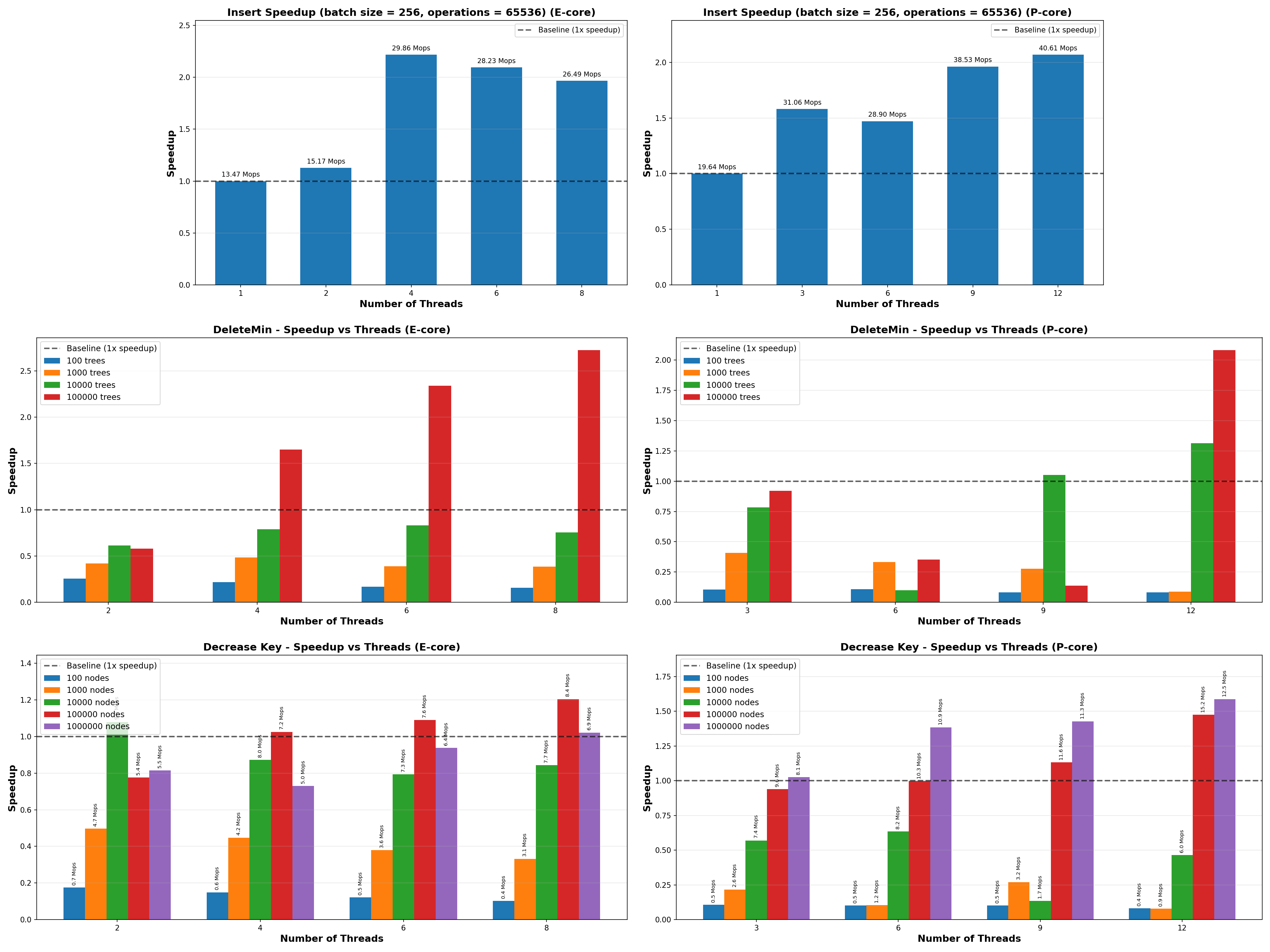 Benchmark of MegaFib on Performance or Efficient Cores
Conclusion
Our results show that Fibonacci heap in parallel is a possible design, but its effectiveness depends strongly on workload composition and synchronization structure. Shared-heap locking approaches help expose the main bottlenecks, but they do not scale well once delete- and decrease-heavy coordination becomes dominant. MegaFib addresses this limitation by distributing heap state across workers, leading to stronger scalability on large workloads and practical benefits in Dijkstra’s algorithm. Batched insertion and tree by tree parallel decrease key operation are introduced for further performance improvements. MageFib’s performance was tested on a heterogeneous computing platform, but the result shows that the heterogeneous programming overhead is not tolerable for our workload. In conclusion, these experiments demonstrate that both algorithmic design and hardware characteristics must be considered carefully when building scalable parallel priority queues such as the Fibonacci heap.
Work Distribution
The work distribution for this project was roughly a 50/50 split among both partners. Zihao worked primarily on implementing the sequential Fibonacci heap baseline, the benchmark testing and two locking & synchronization design. Lemin worked on MegaFib, including all methods implementation, benchmark, dijkstra experiment and heterogeneous. Both team members worked on the experiments, report and poster together, and spent time debugging the whole implementation together.
References
- Michael L. Fredman and Robert Endre Tarjan. “Fibonacci Heaps and Their Uses in Improved Network Optimization Algorithms.” Journal of the ACM, 34(3), 596-615, 1987.
- Thomas H. Cormen, Charles E. Leiserson, and Ronald L. Rivest. Introduction to Algorithms. MIT Press and McGraw-Hill, 1990.
- Qin Huang and William E. Weihl. “An Evaluation of Concurrent Priority Queue Algorithms.” Proceedings of the International Conference on Parallel Processing, 1991.
- Divya Bhattarai. Towards Scalable Parallel Fibonacci Heap Implementation. Master’s thesis, St. Cloud State University, 2018.
- Gerth Stolting Brodal. “Priority Queues with Decreasing Keys.” 12th International Conference on Fun with Algorithms (FUN 2022), LIPIcs 226, 8:1-8:14, 2022.
Fine-Grained Synchronization Procedures
The following pseudocode is adapted from the reference design. Our actual implementation includes several necessary modifications to make the approach work in our setting.
Sectioned Insert
Input: node to_add_node

dummy_list_index <- -1

repeat
    dummy_list_index <- get_random_index()
until dummy_list_locks[dummy_list_index].try_lock() succeeds

dummy_node <- dummy_list[dummy_list_index]

to_add_node->right <- dummy_node->right
to_add_node->left <- dummy_node

if dummy_node->right != nullptr then
    dummy_node->right->left <- to_add_node
end if

dummy_node->right <- to_add_node
dummy_list_locks[dummy_list_index].unlock()
Spill-Over Buffer Refill for One Section
Input: section_index

dummy_list_locks[section_index].lock()
node <- dummy_list[section_index]->right
dummy_list_locks[section_index].unlock()

position <- in_progress_size

while node != nullptr do
    if node->state == UNMARKED then
        in_progress[position] <- node
        i <- position - 1

        while i >= 0 and comparator(in_progress[i + 1]->value,
                                    in_progress[i]->value) do
            swap in_progress[i] and in_progress[i + 1]
            i <- i - 1
        end while

        if position < PROMISING_LIST_SZ + DUMMY_MAX_SZ then
            position <- position + 1
        end if
    end if

    node <- node->right
end while

in_progress_size <- position
Section-by-Section Consolidation
section_index <- -1

repeat
    section_index <- section_index + 1
    initialize local array fibonacci_list[DEGREE_LIMIT] to nullptr

    if consolidate_locks[section_index].try_lock() succeeds then
        head <- dummy_list[section_index]
        curr <- head

        dummy_list_locks[section_index].lock()
        curr <- head->right
        dummy_list_locks[section_index].unlock()

        if curr != nullptr then
            repeat
                if curr->state == UNMARKED then
                    if fibonacci_list[curr->degree] == nullptr then
                        fibonacci_list[curr->degree] <- curr
                    else
                        current_in_list <- nullptr

                        repeat
                            current_in_list <- fibonacci_list[curr->degree]
                            fibonacci_list[curr->degree] <- nullptr
                            curr <- link(curr, current_in_list)
                        until fibonacci_list[curr->degree] == nullptr

                        fibonacci_list[curr->degree] <- curr
                    end if
                else if curr->state == DEAD then
                    remove_and_merge_child(curr)
                    curr <- curr->left
                end if

                if curr != nullptr then
                    curr <- curr->right
                end if
            until curr == nullptr
        end if

        consolidate_locks[section_index].unlock()
    end if
until section_index >= DUMMY_MAX_SZ - 1
Relaxed ExtractMin with Spill-Over and Consolidation
offset <- pointing++

if offset % (3 * PROMISING_LIST_SZ) == PROMISING_LIST_SZ - 2 then
    consolidate()
else if offset % (3 * PROMISING_LIST_SZ) == PROMISING_LIST_SZ - 1 then
    spill_from_all_section()
else if offset % PROMISING_LIST_SZ == 0 then
    count <- count + PROMISING_LIST_SZ
end if

for j <- offset % (3 * PROMISING_LIST_SZ);
    j != count % (3 * PROMISING_LIST_SZ);
    j <- (j + 1) % (3 * PROMISING_LIST_SZ) do

    k <- j

    if promising_list_locks[k].try_lock() succeeds then
        if promising_list[k] != nullptr and
           promising_list[k]->state == PROMISING then

            value <- promising_list[k]->value
            promising_list[k]->state <- DEAD
            promising_list_locks[k].unlock()
            return new Fibonacci heap node containing value
        end if

        promising_list_locks[k].unlock()
    end if
end for

return extractMin()